语义分割

# huggingface

语义分割为图像的每个像素分配一个标签或类。有几种类型的分割，在语义分割的情况下，同一对象的唯一实例之间没有区别。两个对象被赋予相同的标签（例如，“car” 而不是 “car-1” 和 “car-2”）。（这里讲的是同一类物体，比如各种车的么？还是同一个的物体的各个像素点）语义分割的常见实际应用包括训练自动驾驶汽车识别行人和重要的交通信息，识别医学图像中的细胞和异常，以及从卫星图像中监测环境变化。

本指南将向您展示如何在 (SceneParse150)[https://huggingface.co/datasets/scene_parse_150] 数据集上微调 (SegFormer)[https://huggingface.co/docs/transformers/main/en/model_doc/segformer#segformer]。

有关图像分割任务、数据集和指标的详细信息 https://huggingface.co/tasks/image-segmentation

pip install -q datasets transformers evaluate

# Load SceneParse150 dataset

从数据集库中加载 SceneParse150 数据集的前 50 个示例，以便快速训练和测试模型：

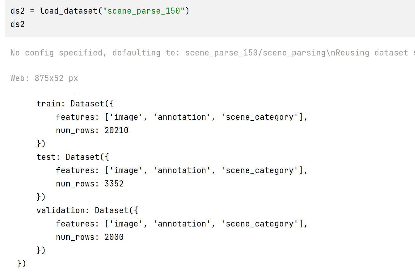
该数据集的大小接近 1G

from datasets import load_dataset

ds = load_dataset("scene_parse_150", split="train[:50]")

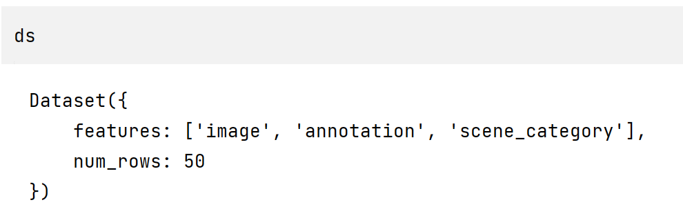
注：使用 load_dataset("scene_parse_150")和load_dataset``("scene_parse_150", split="train[:50]") 都会下载整个数据集，区别只是加载到 ds 中的大小不同。

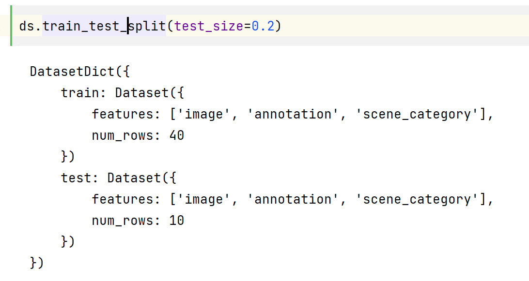
将此数据集拆分为训练集和测试集：

ds = ds.train_test_split(test_size=0.2)
train_ds = ds["train"]
test_ds = ds["test"]

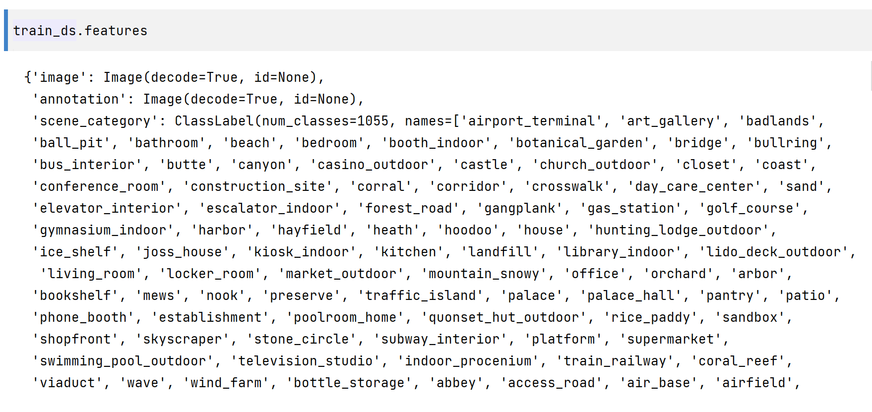
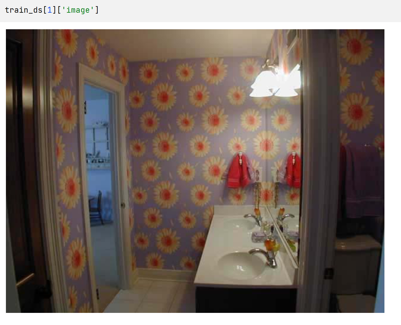
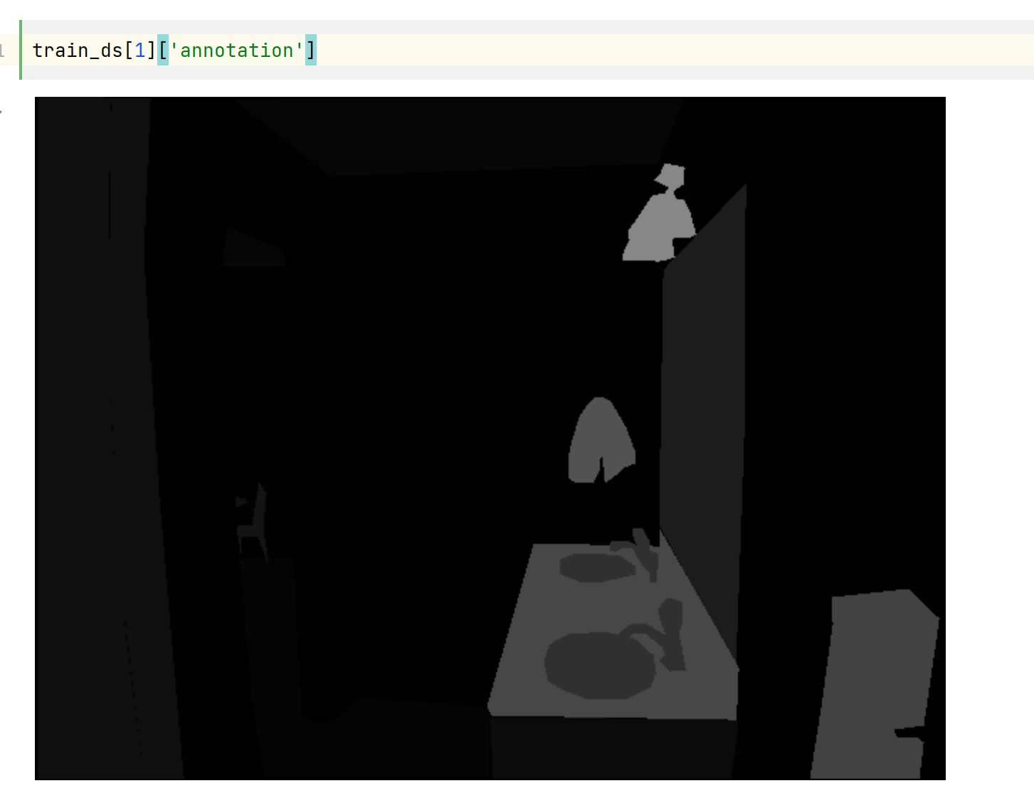
有一个 image 、annotation （这是分割地图或标签）和一个描述图像场景的 scene_category 字段，如 “厨房” 或 “办公室”。在本指南中，您只需要 image 和 annotation，这两者都是 PIL 映像。

image 是三通道的，annotation 是单通道的

image = train_ds[0]['image']
annotation = train_ds[0]['annotation']

print(image, '\n', annotation)

<PIL.JpegImagePlugin.JpegImageFile image mode=RGB size=640x512 at 0x1C69BD73EB0> 
 <PIL.PngImagePlugin.PngImageFile image mode=L size=640x512 at 0x1C69FE91790>

image 和 annotation 的长宽大小是相同的

print(torch.from_numpy(np.array(annotation)).shape)
print(torch.from_numpy(np.array(image)).shape)

torch.Size([512, 640])
torch.Size([512, 640, 3])

annotation 图像上的数值为 0-150，0 表示其他，1-150 为这张表上对应的类别。

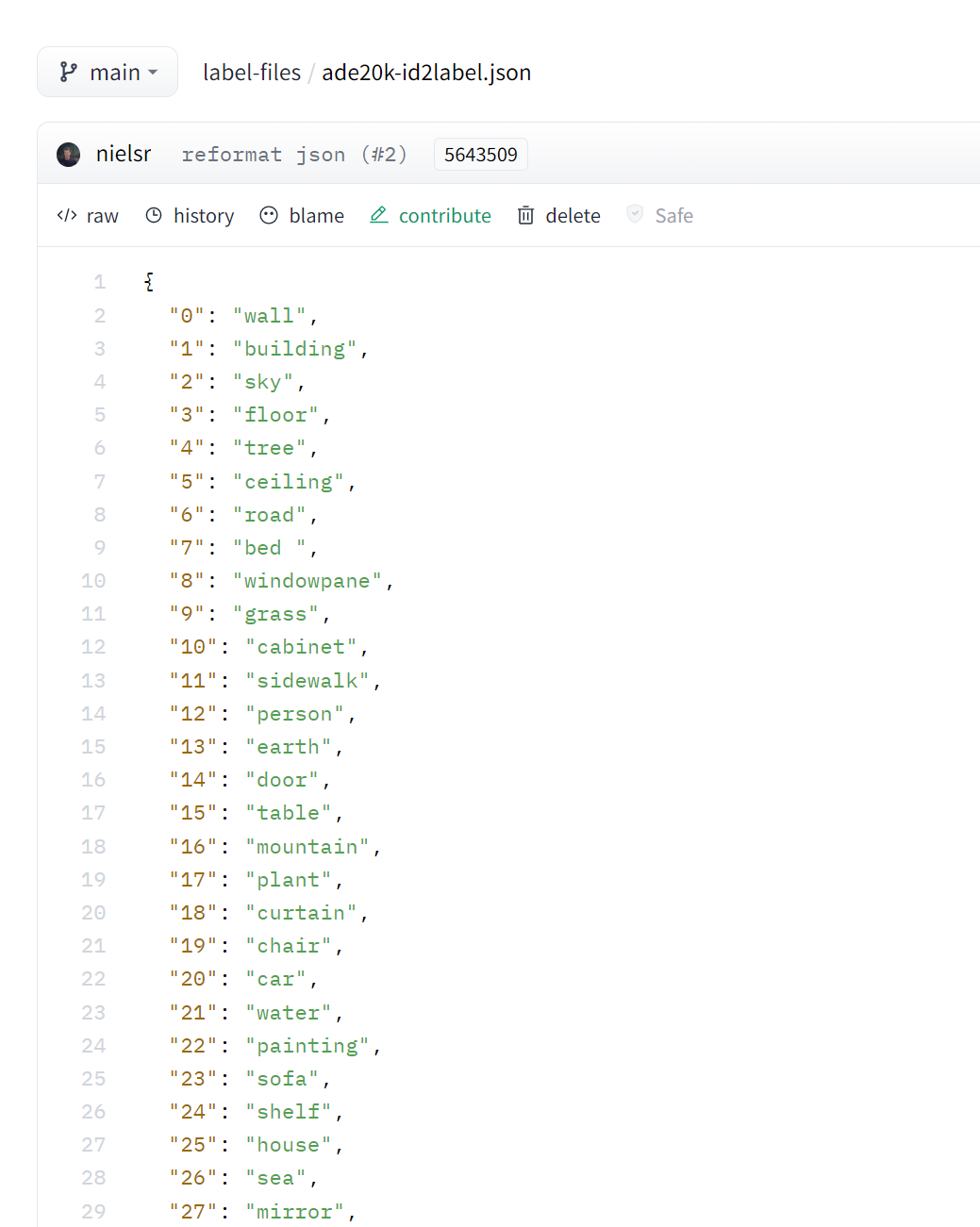
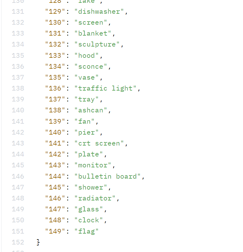
您还需要创建一个将标签 ID 映射到标注分类的字典，这在以后设置模型时会很有用。从 Hub 下载映射并创建 id2label 和 label2id 字典

import json
from huggingface_hub import cached_download, hf_hub_url

repo_id = "datasets/huggingface/label-files"
filename = "ade20k-hf-doc-builder.json"
id2label = json.load(open(cached_download(hf_hub_url(repo_id, filename)), "r"))
id2label = {int(k): v for k, v in id2label.items()}
label2id = {v: k for k, v in id2label.items()}
num_labels = len(id2label)

import json
from huggingface_hub import cached_download, hf_hub_url

repo_id = "datasets/huggingface/label-files"
filename = "ade20k-id2label.json"
id2label = json.load(open(cached_download(hf_hub_url(repo_id, filename)), "r"))
id2label = {int(k): v for k, v in id2label.items()}
label2id = {v: k for k, v in id2label.items()}
num_labels = len(id2label)

id2label 来自的 文件 的两张截图，id 从 0 开始

# Preprocess

接下来，加载 SegFormer 特征提取器以准备模型的图像和注释 annotations。某些数据集（如此数据集）使用零索引作为 background 背景类。但是，后台类不包含在 150 个类中，因此您需要设置 reduce_labels=True，所有标签的 id 值都减 1（此时类别 label 的 id 值从 1 开始编号了）。零索引被替换为 255，因此它被 SegFormer 的 loss 损失函数忽略

from transformers import AutoFeatureExtractor

feature_extractor = AutoFeatureExtractor.from_pretrained("nvidia/mit-b0", reduce_labels=True)

通常将一些数据增强应用于图像数据集，以使模型对过拟合更加可靠（鲁棒性）。在本指南中，您将使用 Torchvision 中的 ColorJitter 函数随机更改图像的颜色属性：

from torchvision.transforms import ColorJitter

jitter = ColorJitter(brightness=0.25, contrast=0.25, saturation=0.25, hue=0.1)

现在创建两个预处理函数来准备模型的图像和注释。这些函数将图像转换为 pixel_values, 将注释 annotations 转换为 labels 。对于训练集，在将图像提供给特征提取器之前应用 jitter。对于测试集，特征提取器裁剪并规范化 images，并且只裁剪 labels，因为在测试期间不应用数据增强。

裁剪不属于数据增强，随机改变图片的颜色属性（如对比度，饱和度等）才属于数据增强。

# 根据官方文档，example_batch是一个字典，每一个键值对中，值是一个列表
def train_transforms(example_batch):
    images = [jitter(x) for x in example_batch["image"]]
    labels = [x for x in example_batch["annotation"]]
    inputs = feature_extractor(images, labels)
    return inputs


def val_transforms(example_batch):
    images = [x for x in example_batch["image"]]
    labels = [x for x in example_batch["annotation"]]
    inputs = feature_extractor(images, labels)
    return inputs

若要对整个数据集应用，请使用 Datasets set_transforml 函数。转换是动态应用的，速度更快，占用的磁盘空间更少

train_ds.set_transform(train_transforms)
test_ds.set_transform(val_transforms)

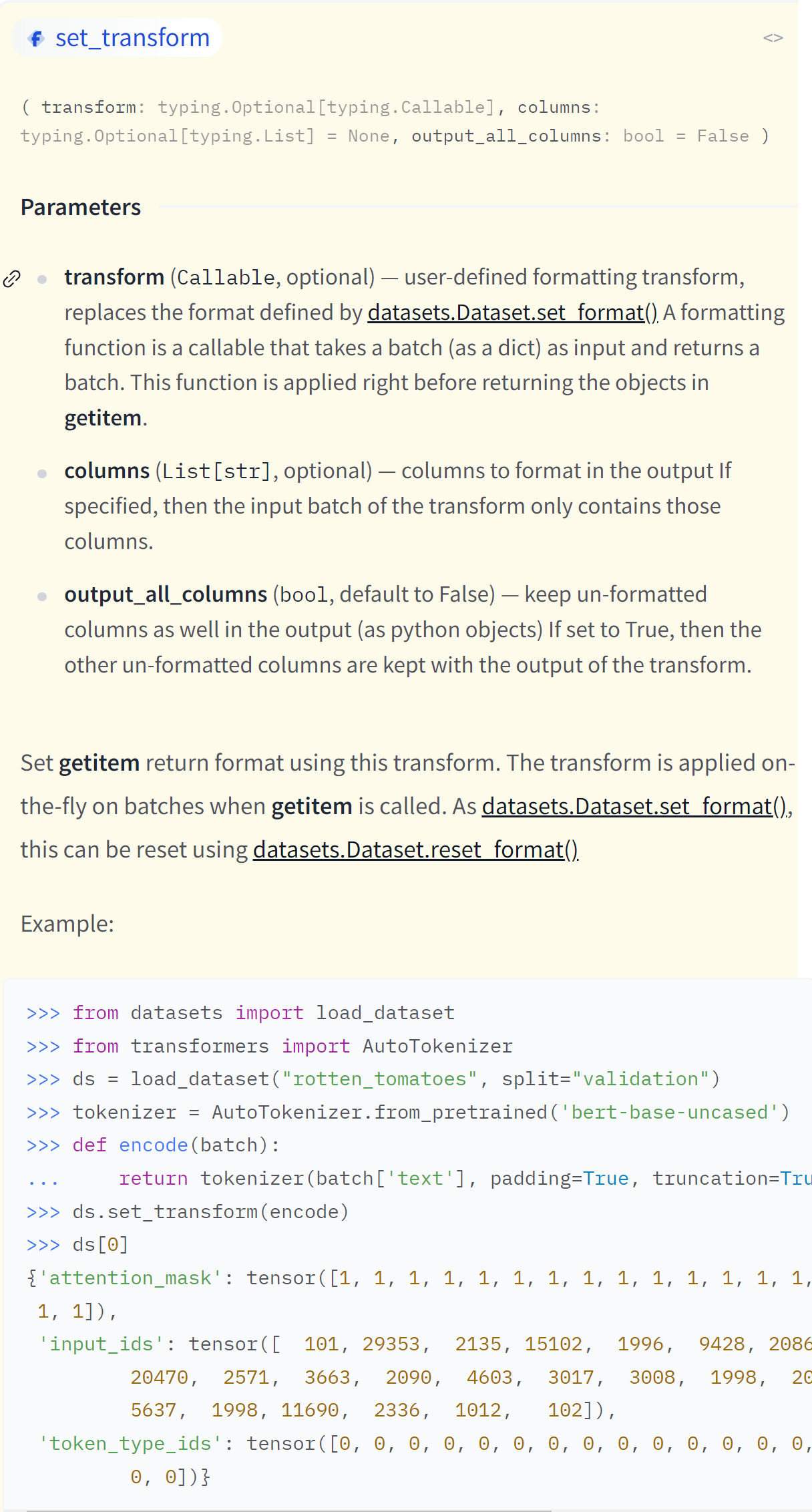
上面只是设置了变换 (set_transform)，还没有对数据集进行变换。

# 从 feature_extractor 的返回值查看它所做的事情（选读）

img1 = train_ds[1]['image']
img2 = train_ds[2]['image']

anno1 = train_ds[1]['annotation']
anno2 = train_ds[2]['annotation']

res = feature_extractor(img1, anno1)
res.keys()  # dict_keys(['pixel_values', 'labels'])

pixel_values = res['pixel_values']
len(pixel_values) # 1 
# pixel_values 是一个列表，说明feature_extractor是进行批处理的，将每个图像处理的结果整合成一个列表

# feature_extractor调整了图像的大小，因为模型只能接受固定大小的图片吧
pixel_values[0].shape # (3, 512, 512)
labels[0].shape # (512, 512)

# feature_extractor 更改了图片中的像素值，应该是对图片进行了某种处理（类似卷积池化等操作吧）
torch.from_numpy(np.array(anno1)).max() # tensor(82, dtype=torch.uint8)
torch.from_numpy(np.array(pixel_values[0])).max() # tensor(2.6400)

批处理时

res = feature_extractor([img1, img2], [anno1, anno2])

# Train

使用 AutoModelForSemanticSegmentation 加载 SegFormer，并向模型传递标签 ID 和标签类之间的映射：

from transformers import AutoModelForSemanticSegmentation

pretrained_model_name = "nvidia/mit-b0"
model = AutoModelForSemanticSegmentation.from_pretrained(
    pretrained_model_name, id2label=id2label, label2id=label2id
)

在 TrainingArguments 中定义训练超参数。重要的是不要删除未使用的列，因为这会删除 image 列。如果没有 image 列，则无法创建 pixel_values。设置 remove_unused_columns=False 为防止此行为

若要将命名空间下的模型保存并推送到 Hub，请设置 push_to_hub=True

from transformers import TrainingArguments

training_args = TrainingArguments(
    output_dir="segformer-b0-scene-parse-150",
    learning_rate=6e-5,
    num_train_epochs=50,
    per_device_train_batch_size=2,
    per_device_eval_batch_size=2,
    save_total_limit=3,
    evaluation_strategy="steps",
    save_strategy="steps",
    save_steps=20,
    eval_steps=20,
    logging_steps=1,
    eval_accumulation_steps=5,
    remove_unused_columns=False,
    push_to_hub=True,
)

若要在训练期间评估模型性能，需要创建一个函数来计算和报告指标。对于语义分割，通常计算平均并集交点 mean Intersection over Union （IoU）。平均 IoU 测量预测和地面实况分割地图之间的重叠区域。

从 Evaluate 库加载平均 IoU：

import evaluate

metric = evaluate.load("mean_iou")

然后创建一个函数来计算指标。您的预测需要先转换为 logits，然后重新调整大小以匹配标签的大小，然后才能调用计算：

def compute_metrics(eval_pred):
    with torch.no_grad():
        logits, labels = eval_pred
        logits_tensor = torch.from_numpy(logits)
        logits_tensor = nn.functional.interpolate(
            logits_tensor,
            size=labels.shape[-2:],
            mode="bilinear",
            align_corners=False,
        ).argmax(dim=1)

        pred_labels = logits_tensor.detach().cpu().numpy()
        metrics = metric.compute(
            predictions=pred_labels,
            references=labels,
            num_labels=num_labels,
            ignore_index=255,
            reduce_labels=False,
        )
        for key, value in metrics.items():
            if type(value) is np.ndarray:
                metrics[key] = value.tolist()
        return metrics

将模型、训练参数、数据集和指标函数传递给 Trainer:：

from transformers import Trainer

trainer = Trainer(
    model=model,
    args=training_args,
    train_dataset=train_ds,
    eval_dataset=test_ds,
    compute_metrics=compute_metrics,
)

# Inference 推理

加载图像以进行推理：

image = ds[0]["image"]
image

使用特征提取器处理图像，并将 pixel_values 置于 GPU 上

device = torch.device("cuda" if torch.cuda.is_available() else "cpu")  # use GPU if available, otherwise use a CPU
encoding = feature_extractor(image, return_tensors="pt")
pixel_values = encoding.pixel_values.to(device)

将输入传递给模型并返回 logits

outputs = model(pixel_values=pixel_values)
logits = outputs.logits.cpu()

查看 outputs

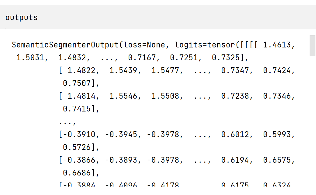
查看 logits

logits 已经是 tensor 类型了

logits.shape # torch.Size([1, 150, 128, 128])

logits.dtype # torch.float32

第二维度的 150 正好对应上面所述的 150 种 label 类别，对应位置上的值应该类似是该点所属类别的概率，（但是奇怪的是每个位置上的 150 个值进行求和，所得结果却不是 1，无论是对 logits 还是 upsampled_logits），

l = []

for i in range(150):

    l.append(logits[0][i][0][0])

sum = 0

for i in range(len(l)):

    sum += l[i]

print(sum)

接下来，将 logits 重新缩放到原始映像大小：

upsampled_logits = nn.functional.interpolate(
    logits,
    size=image.size[::-1],
    mode="bilinear",
    align_corners=False,
)

pred_seg = upsampled_logits.argmax(dim=1)[0]

若要可视化结果，请加载将每个类映射到其 RGB 值的数据集调色板。然后，您可以组合并绘制图像和预测分割图：

import matplotlib.pyplot as plt

color_seg = np.zeros((pred_seg.shape[0], pred_seg.shape[1], 3), dtype=np.uint8)
palette = np.array(ade_palette())
for label, color in enumerate(palette):
    color_seg[pred_seg == label, :] = color
color_seg = color_seg[..., ::-1]  # convert to BGR

img = np.array(image) * 0.5 + color_seg * 0.5  # plot the image with the segmentation map
img = img.astype(np.uint8)

plt.figure(figsize=(15, 10))
plt.imshow(img)
plt.show()

上面的 ade_palette 不知道从哪里来的